数据挖掘入门项目二手交易车价格预测之建模调参

04-11 1019阅读

文章目录

目标
步骤

1. 调整数据类型，减少数据在内存中占用的空间
2. 使用线性回归来简单建模
3. 五折交叉验证
4. 模拟真实业务情况
5. 绘制学习率曲线与验证曲线
6. 嵌入式特征选择
6. 非线性模型
7. 模型调参

（1）贪心调参
（2）Grid Search 调参
（3）贝叶斯调参

总结

本文数据集来自阿里天池：https://tianchi.aliyun.com/competition/entrance/231784/information

主要参考了Datawhale的整个操作流程：https://tianchi.aliyun.com/notebook/95460

小编也是第一次接触数据挖掘，所以先跟着Datawhale写的教程操作了一遍，不懂的地方加了一点点自己的理解，感谢Datawhale！

目标

了解常用的机器学习模型，并掌握机器学习模型的建模与调参流程

步骤

1. 调整数据类型，减少数据在内存中占用的空间

具体方法定义如下：

对每一列循环，将每一列的转化为对应的数据类型，在不损失数据的情况下，尽可能地减少DataFrame中每列的内存占用

def reduce_mem_usage(df):
    """ iterate through all the columns of a dataframe and modify the data type
        to reduce memory usage.        
    """
    start_mem = df.memory_usage().sum()  # memory_usage() 方法返回每一列的内存使用情况，sum() 将它们相加。
    print('Memory usage of dataframe is {:.2f} MB'.format(start_mem))
    # 对每一列循环
    for col in df.columns:
        col_type = df[col].dtype # 获取列类型
        if col_type != object:
            # 获取当前列的最小值和最大值
            c_min = df[col].min()
            c_max = df[col].max()
            if str(col_type)[:3] == 'int':
                # np.int8 是 NumPy 中表示 8 位整数的数据类型。
                # np.iinfo(np.int8) 返回一个描述 np.int8 数据类型的信息对象。
                # .min 是该信息对象的一个属性，用于获取该数据类型的最小值。
                if c_min > np.iinfo(np.int8).min and c_max  np.iinfo(np.int16).min and c_max  np.iinfo(np.int32).min and c_max  np.iinfo(np.int64).min and c_max  np.finfo(np.float16).min and c_max  np.finfo(np.float32).min and c_max  
调用上述函数查看效果：
其中，data_for_tree.csv保存的是我们在特征工程步骤中简单处理过的特征 
sample_feature = reduce_mem_usage(pd.read_csv('data_for_tree.csv'))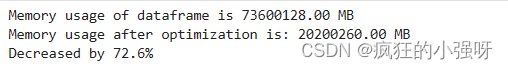
 
 
2. 使用线性回归来简单建模 
因为上述特征当时是为树模型分析保存的，所以没有对空值进行处理，这里简单处理一下 
sample_feature.head()
 
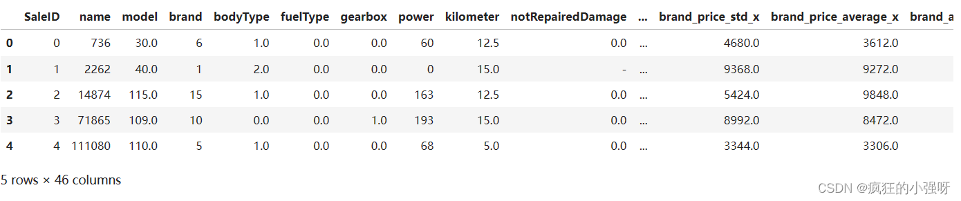
可以看到notRepairedDamage这一列有异常值‘-’： 
sample_feature = sample_feature.dropna().replace('-', 0).reset_index(drop=True)
sample_feature['notRepairedDamage'] = sample_feature['notRepairedDamage'].astype(np.float32)
 
建立训练数据和标签： 
train_X = sample_feature.drop('price',axis=1)
train_y = sample_feature['price']
 
简单建模： 
from sklearn.linear_model import LinearRegression
model = LinearRegression()
model = model.fit(train_X, train_y)
'intercept:'+ str(model.intercept_) # 这一行代码用于输出模型的截距（即常数项）
sorted(dict(zip(sample_feature.columns, model.coef_)).items(), key=lambda x:x[1], reverse=True) # 这行代码是用于输出模型的系数，并按照系数的大小进行排序
# sample_feature.columns 是特征的列名。
# model.coef_ 是线性回归模型的系数。
# zip(sample_feature.columns, model.coef_) 将特征列名与对应的系数打包成元组。
# dict(...) 将打包好的元组转换为字典。
# sorted(..., key=lambda x:x[1], reverse=True) 对字典按照值（系数）进行降序排序。
 
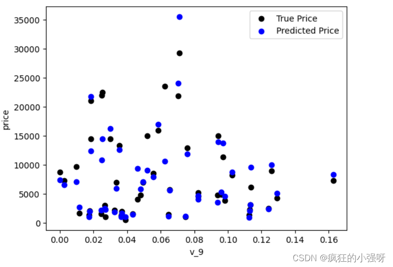
画图查看真实值与预测值之间的差距： 
from matplotlib import pyplot as plt
subsample_index = np.random.randint(low=0, high=len(train_y), size=50) # 从训练数据中随机选择 50 个样本的索引
plt.scatter(train_X['v_9'][subsample_index], train_y[subsample_index], color='black') # 绘制真实价格与特征 'v_9' 之间的散点图
plt.scatter(train_X['v_9'][subsample_index], model.predict(train_X.loc[subsample_index]), color='blue') # 绘制模型预测价格与特征 'v_9' 之间的散点图
plt.xlabel('v_9')
plt.ylabel('price')
plt.legend(['True Price','Predicted Price'],loc='upper right')
print('The predicted price is obvious different from true price')
plt.show()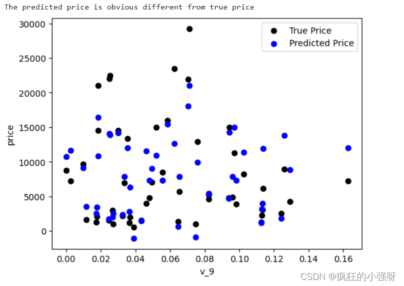
 
通过作图我们发现数据的标签（price）呈现长尾分布，不利于我们的建模预测。
对标签进行进一步分析：
画图显示标签的分布：左边是所有标签数据的一个分布，右边是去掉最大的10%标签数据之后的一个分布 
import seaborn as sns
print('It is clear to see the price shows a typical exponential distribution')
plt.figure(figsize=(15,5))
plt.subplot(1,2,1) # 创建一个包含 1 行 2 列的子图，并将当前子图设置为第一个子图
sns.distplot(train_y) # 显示价格数据的直方图以及拟合的密度曲线
plt.subplot(1,2,2)
# quantile 函数来计算价格数据的第 90%分位数，然后通过布尔索引选取低于第 90 百分位数的价格数据
sns.distplot(train_y[train_y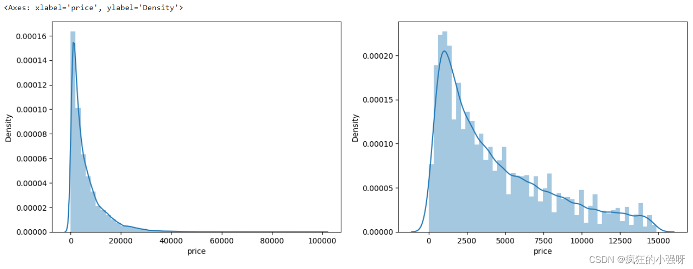  
对标签进行 log(x+1) 变换，使标签贴近于正态分布： 
train_y_ln = np.log(train_y + 1)
 
显示log变化之后的数据分布： 
import seaborn as sns
print('The transformed price seems like normal distribution')
plt.figure(figsize=(15,5))
plt.subplot(1,2,1)
sns.distplot(train_y_ln)
plt.subplot(1,2,2)
sns.distplot(train_y_ln[train_y_ln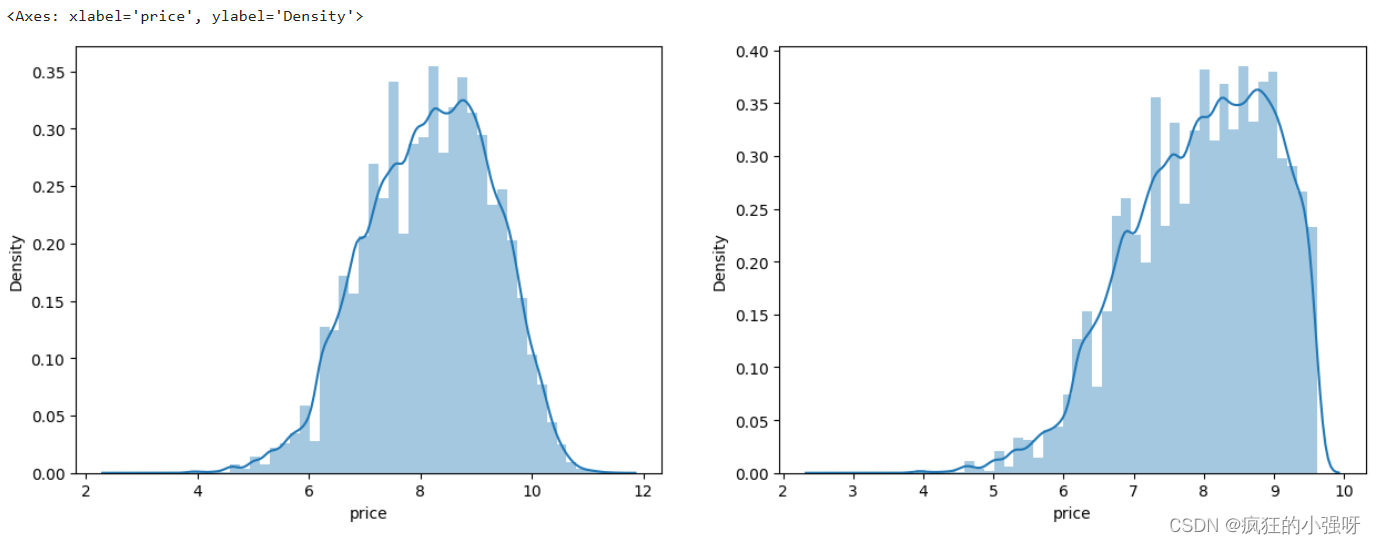  
然后我们重新训练，再可视化 
model = model.fit(train_X, train_y_ln)
print('intercept:'+ str(model.intercept_))
sorted(dict(zip(continuous_feature_names, model.coef_)).items(), key=lambda x:x[1], reverse=True)
plt.scatter(train_X['v_9'][subsample_index], train_y[subsample_index], color='black')
plt.scatter(train_X['v_9'][subsample_index], np.exp(model.predict(train_X.loc[subsample_index])), color='blue')
plt.xlabel('v_9')
plt.ylabel('price')
plt.legend(['True Price','Predicted Price'],loc='upper right')
print('The predicted price seems normal after np.log transforming')
plt.show()
 
可以看出结果要比上面的好一点：
 
3. 五折交叉验证 
 
 在使用训练集对参数进行训练的时候，一般会将整个训练集分为三个部分：训练集（train_set），评估集（valid_set），测试集（test_set）这三个部分。这其实是为了保证训练效果而特意设置的。

测试集很好理解，其实就是完全不参与训练的数据，仅仅用来观测测试效果的数据。

在实际的训练中，训练的结果对于训练集的拟合程度通常还是挺好的（初始条件敏感），但是对于训练集之外的数据的拟合程度通常就不那么令人满意了。因此我们通常并不会把所有的数据集都拿来训练，而是分出一部分来（这一部分不参加训练）对训练集生成的参数进行测试，相对客观的判断这些参数对训练集之外的数据的符合程度。这种思想就称为交叉验证（Cross Validation）

（1）使用线性回归模型，对未处理标签的特征数据进行五折交叉验证

from sklearn.model_selection import cross_val_score
from sklearn.metrics import mean_absolute_error,  make_scorer
# 下面这个函数主要实现对参数进行对数转换输入目标函数
def log_transfer(func):
    def wrapper(y, yhat):
        # np.nan_to_num 函数用于将对数转换后可能出现的 NaN 值转换为 0
        result = func(np.log(y), np.nan_to_num(np.log(yhat)))
        return result
    # 返回内部函数 wrapper，这是一个对原始函数的包装器，它将对传入的参数进行对数转换后再调用原始函数
    return wrapper
# 计算5折交叉验证得分
scores = cross_val_score(model, X=train_X, y=train_y, verbose=1, cv = 5, scoring=make_scorer(log_transfer(mean_absolute_error)))
# model 是要评估的模型对象。
# train_X 是训练数据的特征，train_y 是训练数据的目标变量。
# verbose=1 设置为 1 时表示打印详细信息。
# cv=5 表示进行 5 折交叉验证。
# scoring=make_scorer(log_transfer(mean_absolute_error)) 指定了评分标准
# 使用了 make_scorer 函数将一个自定义的评分函数 log_transfer(mean_absolute_error) 转换为一个可用于评分的评估器。
# log_transfer(mean_absolute_error) 这一步的作用就是将真实值和预测值在输入到mean_absolute_error之前进行log转换
# mean_absolute_error 是一个回归问题中常用的评估指标，用于衡量预测值与实际值之间的平均绝对误差
print('AVG:', np.mean(scores))

结果展示：

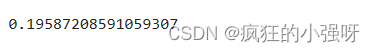
使用线性回归模型，对处理过标签的特征数据进行五折交叉验证：

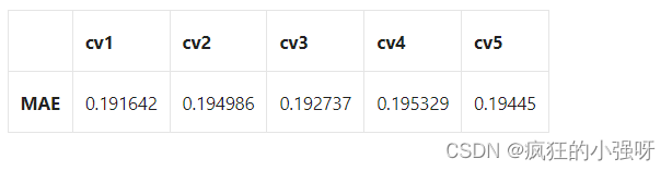
scores = cross_val_score(model, X=train_X, y=train_y_ln, verbose=1, cv = 5, scoring=make_scorer(mean_absolute_error))
print('AVG:', np.mean(scores))

结果展示：

可以看见，调整之后的数据，误差明显变小

查看scores：

scores = pd.DataFrame(scores.reshape(1,-1))
scores.columns = ['cv' + str(x) for x in range(1, 6)]
scores.index = ['MAE']
scores

4. 模拟真实业务情况

交叉验证在某些与时间相关的数据集上可能反映了不真实的情况，比如我们不能通过2018年的二手车价格来预测2017年的二手车价格。这个时候我们可以采用时间顺序对数据集进行分隔。在本例中，我们可以选用靠前时间的4/5样本当作训练集，靠后时间的1/5当作验证集

具体操作如下：

import datetime
sample_feature = sample_feature.reset_index(drop=True)
split_point = len(sample_feature) // 5 * 4
train = sample_feature.loc[:split_point].dropna()
val = sample_feature.loc[split_point:].dropna()
train_X = train.drop('price',axis=1)
train_y_ln = np.log(train['price'] + 1)
val_X = val.drop('price',axis=1)
val_y_ln = np.log(val['price'] + 1)
model = model.fit(train_X, train_y_ln)
mean_absolute_error(val_y_ln, model.predict(val_X))

结果展示：

5. 绘制学习率曲线与验证曲线

def plot_learning_curve(estimator, title, X, y, ylim=None, cv=None,n_jobs=1, train_size=np.linspace(.1, 1.0, 5 )): 
    """
    模型估计器 estimator
    图的标题 title
    特征数据 X
    目标数据 y
    y轴的范围 ylim
    交叉验证分割策略 cv
    并行运行的作业数 n_jobs 
    训练样本的大小 train_size
    """
    plt.figure()  
    plt.title(title)  
    if ylim is not None:  
        plt.ylim(*ylim)  # 设置 y 轴的范围为 ylim
    plt.xlabel('Training example')  
    plt.ylabel('score')  
    # 使用 learning_curve 函数计算学习曲线的训练集得分和交叉验证集得分
    train_sizes, train_scores, test_scores = learning_curve(estimator, X, y, cv=cv, n_jobs=n_jobs, train_sizes=train_size, scoring = make_scorer(mean_absolute_error))  
    train_scores_mean = np.mean(train_scores, axis=1)  # 计算训练集得分的均值
    train_scores_std = np.std(train_scores, axis=1)  # 计算训练集得分的标准差
    test_scores_mean = np.mean(test_scores, axis=1)  
    test_scores_std = np.std(test_scores, axis=1)  
    plt.grid()#区域  
    # 使用红色填充训练集得分的方差范围
    plt.fill_between(train_sizes, train_scores_mean - train_scores_std,  
                     train_scores_mean + train_scores_std, alpha=0.1,  
                     color="r")  
    # 使用绿色填充交叉验证集得分的方差范围
    plt.fill_between(train_sizes, test_scores_mean - test_scores_std,  
                     test_scores_mean + test_scores_std, alpha=0.1,  
                     color="g")  
    # 绘制训练集得分曲线
    plt.plot(train_sizes, train_scores_mean, 'o-', color='r',  
             label="Training score")  
    # 绘制交叉验证集得分曲线
    plt.plot(train_sizes, test_scores_mean,'o-',color="g",  
             label="Cross-validation score")  
    plt.legend(loc="best")  
    return plt 
plot_learning_curve(LinearRegression(), 'Liner_model', train_X[:1000], train_y_ln[:1000], ylim=(0.0, 0.5), cv=5, n_jobs=1)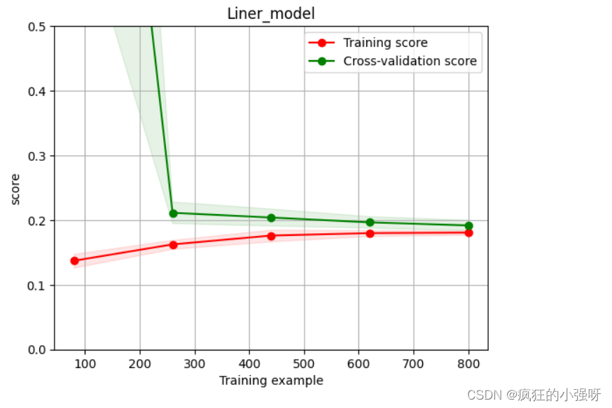

6. 嵌入式特征选择

在过滤式和包裹式特征选择方法中，特征选择过程与学习器训练过程有明显的分别。而嵌入式特征选择在学习器训练过程中自动地进行特征选择。嵌入式选择最常用的是L1正则化与L2正则化。在对线性回归模型加入两种正则化方法后，他们分别变成了岭回归与Lasso回归

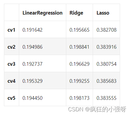
对上述三种模型进行交叉验证训练，并对比结果：

from sklearn.linear_model import LinearRegression
from sklearn.linear_model import Ridge
from sklearn.linear_model import Lasso
# 创建一个模型实力列表
models = [LinearRegression(),
          Ridge(),
          Lasso()]
result = dict()
for model in models:
    model_name = str(model)[:-2] # 获取模型名称
    # 训练模型
    scores = cross_val_score(model, X=train_X, y=train_y_ln, verbose=0, cv = 5, scoring=make_scorer(mean_absolute_error))
    # 收集各模型训练得分
    result[model_name] = scores
    print(model_name + ' is finished')
result = pd.DataFrame(result)
result.index = ['cv' + str(x) for x in range(1, 6)]
result

结果展示：

分别对三个模型训练得到的参数进行分析：

一般线性回归

import seaborn as sns
model = LinearRegression().fit(train_X, train_y_ln)
print('intercept:', model.intercept_)
# 组合数据
data = pd.DataFrame({'coef_abs': abs(model.coef_), 'feature': train_X.columns})
# 画图
sns.barplot(x='coef_abs', y='feature', data=data)

展示：

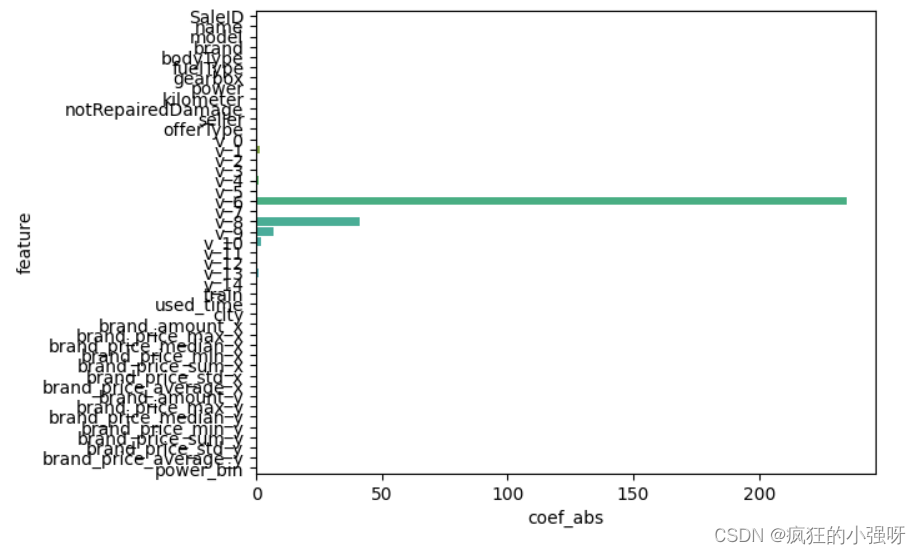
岭回归

L2正则化在拟合过程中通常都倾向于让权值尽可能小，最后构造一个所有参数都比较小的模型。因为一般认为参数值小的模型比较简单，能适应不同的数据集，也在一定程度上避免了过拟合现象。可以设想一下对于一个线性回归方程，若参数很大，那么只要数据偏移一点点，就会对结果造成很大的影响；但如果参数足够小，数据偏移得多一点也不会对结果造成什么影响，专业一点的说法是『抗扰动能力强』

import seaborn as sns
model = Ridge().fit(train_X, train_y_ln)
print('intercept:', model.intercept_)
# 组合数据
data = pd.DataFrame({'coef_abs': abs(model.coef_), 'feature': train_X.columns})
sns.barplot(x='coef_abs', y='feature', data=data)

展示：

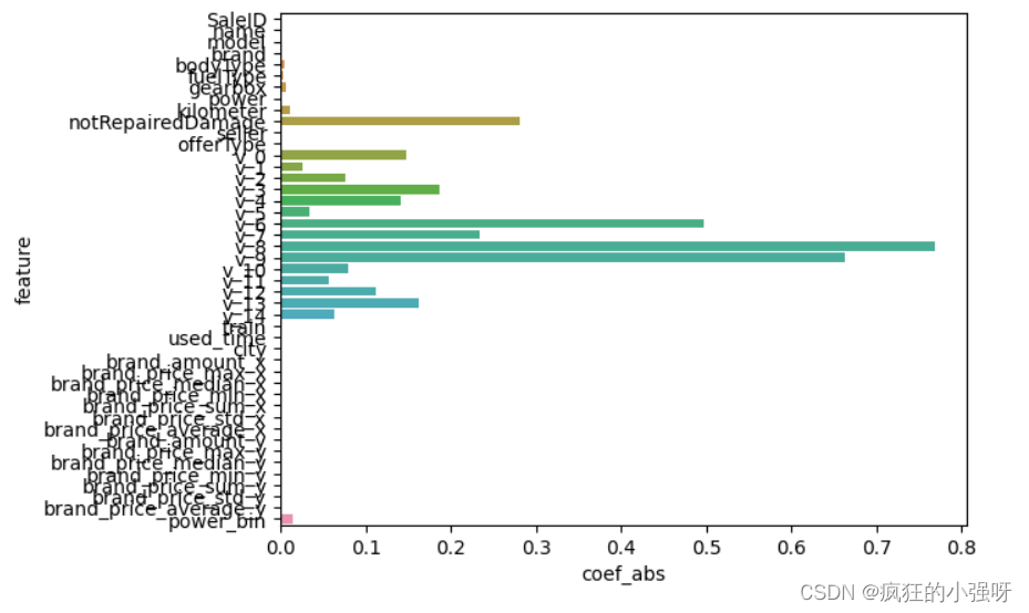
Lasso回归

L1正则化有助于生成一个稀疏权值矩阵，进而可以用于特征选择

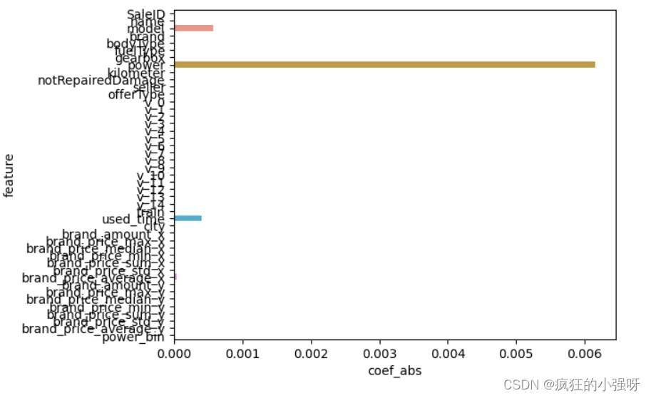
import seaborn as sns
model = Lasso().fit(train_X, train_y_ln)
print('intercept:', model.intercept_)
# 组合数据
data = pd.DataFrame({'coef_abs': abs(model.coef_), 'feature': train_X.columns})
sns.barplot(x='coef_abs', y='feature', data=data)

展示：

在这里我们可以看到power、used_time等特征非常重要

6. 非线性模型

决策树通过信息熵或GINI指数选择分裂节点时，优先选择的分裂特征也更加重要，这同样是一种特征选择的方法。XGBoost与LightGBM模型中的model_importance指标正是基于此计算的

下面我们选择部分模型进行对比：

from sklearn.linear_model import LinearRegression
from sklearn.svm import SVC
from sklearn.tree import DecisionTreeRegressor
from sklearn.ensemble import RandomForestRegressor
from sklearn.ensemble import GradientBoostingRegressor
from sklearn.neural_network import MLPRegressor
from xgboost.sklearn import XGBRegressor
from lightgbm.sklearn import LGBMRegressor
models = [LinearRegression(),
          DecisionTreeRegressor(),
          RandomForestRegressor(),
          GradientBoostingRegressor(),
          MLPRegressor(solver='lbfgs', max_iter=100), 
          XGBRegressor(n_estimators = 100, objective='reg:squarederror'), 
          LGBMRegressor(n_estimators = 100)]
result = dict()
for model in models:
    model_name = str(model).split('(')[0]
    scores = cross_val_score(model, X=train_X, y=train_y_ln, verbose=0, cv = 5, scoring=make_scorer(mean_absolute_error))
    result[model_name] = scores
    print(model_name + ' is finished')
result = pd.DataFrame(result)
result.index = ['cv' + str(x) for x in range(1, 6)]
result

结果：

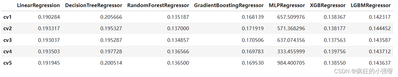
可以看到随机森林模型在每一个fold中均取得了更好的效果！！！

7. 模型调参

在这里主要介绍三种调参方法

（1）贪心调参

所谓贪心算法是指，在对问题求解时，总是做出在当前看来是最好的选择。也就是说，不从整体最优上加以考虑，它所做出的仅仅是在某种意义上的局部最优解。

以lightgbm模型为例：

## LGB的参数集合：
# 损失函数
objective = ['regression', 'regression_l1', 'mape', 'huber', 'fair']
# 叶子节点数
num_leaves = [3,5,10,15,20,40, 55]
# 最大深度
max_depth = [3,5,10,15,20,40, 55]
bagging_fraction = []
feature_fraction = []
drop_rate = []
best_obj = dict()
# 计算不同选择下对应结果，其中 score最小时为最优结果
for obj in objective:
    model = LGBMRegressor(objective=obj)
    score = np.mean(cross_val_score(model, X=train_X, y=train_y_ln, verbose=0, cv = 5, scoring=make_scorer(mean_absolute_error)))
    best_obj[obj] = score
    
best_leaves = dict()
for leaves in num_leaves:
    model = LGBMRegressor(objective=min(best_obj.items(), key=lambda x:x[1])[0], num_leaves=leaves)
    score = np.mean(cross_val_score(model, X=train_X, y=train_y_ln, verbose=0, cv = 5, scoring=make_scorer(mean_absolute_error)))
    best_leaves[leaves] = score
    
best_depth = dict()
for depth in max_depth:
    model = LGBMRegressor(objective=min(best_obj.items(), key=lambda x:x[1])[0],
                          num_leaves=min(best_leaves.items(), key=lambda x:x[1])[0],
                          max_depth=depth)
    score = np.mean(cross_val_score(model, X=train_X, y=train_y_ln, verbose=0, cv = 5, scoring=make_scorer(mean_absolute_error)))
    best_depth[depth] = score
# 画出各选择下，损失的变化
sns.lineplot(x=['0_initial','1_turning_obj','2_turning_leaves','3_turning_depth'], y=[0.143 ,min(best_obj.values()), min(best_leaves.values()), min(best_depth.values())])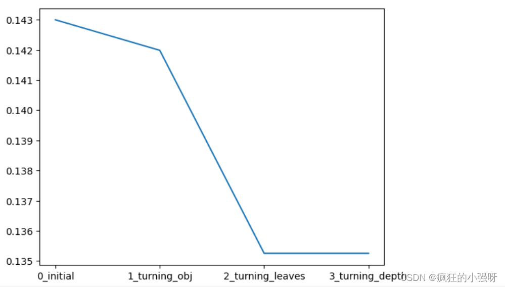

（2）Grid Search 调参

GridSearchCV：一种调参的方法，当你算法模型效果不是很好时，可以通过该方法来调整参数，通过循环遍历，尝试每一种参数组合，返回最好的得分值的参数组合

from sklearn.model_selection import GridSearchCV
parameters = {'objective': objective , 'num_leaves': num_leaves, 'max_depth': max_depth}
model = LGBMRegressor()
clf = GridSearchCV(model, parameters, cv=5)
clf = clf.fit(train_X, train_y_ln)
clf.best_params_

得到的最佳参数为：{'max_depth': 10, 'num_leaves': 55, 'objective': 'huber'}

我们再用最佳参数来训练模型：

model = LGBMRegressor(objective='huber',
                          num_leaves=55,
                          max_depth=10)
np.mean(cross_val_score(model, X=train_X, y=train_y_ln, verbose=0, cv = 5, scoring=make_scorer(mean_absolute_error)))

结果跟之前的调参是相当的：

（3）贝叶斯调参

贝叶斯优化通过基于目标函数的过去评估结果建立替代函数（概率模型），来找到最小化目标函数的值。贝叶斯方法与随机或网格搜索的不同之处在于，它在尝试下一组超参数时，会参考之前的评估结果，因此可以省去很多无用功。

from bayes_opt import BayesianOptimization
def rf_cv(num_leaves, max_depth, subsample, min_child_samples):
    #num_leaves: 决策树上的叶子节点数量。较大的值可以提高模型的复杂度，但也容易导致过拟合。
    # max_depth: 决策树的最大深度。控制树的深度可以限制模型的复杂度，有助于防止过拟合。
    # subsample: 训练数据的子样本比例。该参数可以用来控制每次迭代时使用的数据量，有助于加速训练过程并提高模型的泛化能力。
    # min_child_samples: 每个叶子节点所需的最小样本数。通过限制叶子节点中的样本数量，可以控制树的生长，避免过拟合。
    val = cross_val_score(
        LGBMRegressor(objective = 'regression_l1',
            num_leaves=int(num_leaves),
            max_depth=int(max_depth),
            subsample = subsample,
            min_child_samples = int(min_child_samples)
        ),
        X=train_X, y=train_y_ln, verbose=0, cv = 5, scoring=make_scorer(mean_absolute_error)
    ).mean()
    return 1 - val
    
rf_bo = BayesianOptimization(
    rf_cv,
    {
    'num_leaves': (2, 100),
    'max_depth': (2, 100),
    'subsample': (0.1, 1),
    'min_child_samples' : (2, 100)
    }
)
# 最大化 rf_cv 函数返回的值，即最小化负的平均绝对误差
rf_bo.maximize()

结果：

1 - rf_bo.max['target']

总结

上述我们主要通过log转换、正则化、模型选择、参数微调等方法来提高预测的精度
最后附上一些学习链接供大家参考：
线性回归模型：https://zhuanlan.zhihu.com/p/49480391
决策树模型：https://zhuanlan.zhihu.com/p/65304798
GBDT模型：https://zhuanlan.zhihu.com/p/45145899
XGBoost模型：https://zhuanlan.zhihu.com/p/86816771
LightGBM模型：https://zhuanlan.zhihu.com/p/89360721
用简单易懂的语言描述「过拟合 overfitting」？https://www.zhihu.com/question/32246256/answer/55320482
模型复杂度与模型的泛化能力：http://yangyingming.com/article/434/
正则化的直观理解：https://blog.csdn.net/jinping_shi/article/details/52433975
贪心算法： https://www.jianshu.com/p/ab89df9759c8
网格调参： https://blog.csdn.net/weixin_43172660/article/details/83032029
贝叶斯调参： https://blog.csdn.net/linxid/article/details/81189154

VPS购买请点击我

数据挖掘入门项目二手交易车价格预测之建模调参

文章目录

目标

步骤

1. 调整数据类型，减少数据在内存中占用的空间

4. 模拟真实业务情况

5. 绘制学习率曲线与验证曲线

6. 嵌入式特征选择

6. 非线性模型

7. 模型调参

（1）贪心调参

（2）Grid Search 调参

（3）贝叶斯调参

总结

相关阅读

C#连接Mysql数据库详细教程（内附Mysql及Navicat)

Spring Boot 禁用 Swagger 的三种方式

打包部署若依SpringBoot后端和Vue前端

2024最新首发，全网最全 Spring Boot 学习宝典(附思维导图)

目录[+]

文章目录

目标

步骤

1. 调整数据类型，减少数据在内存中占用的空间

2. 使用线性回归来简单建模

3. 五折交叉验证

4. 模拟真实业务情况

5. 绘制学习率曲线与验证曲线

6. 嵌入式特征选择

6. 非线性模型

7. 模型调参

（1） 贪心调参

（2）Grid Search 调参

（3）贝叶斯调参

总结

相关阅读

C#连接Mysql数据库详细教程（内附Mysql及Navicat)

Spring Boot 禁用 Swagger 的三种方式

打包部署若依SpringBoot后端和Vue前端

2024最新首发，全网最全 Spring Boot 学习宝典(附思维导图)

目录[+]

（1）贪心调参